Spline Regression [Piecewise polynomials]
Mostly, we have two ways to fit a regression line to our data:
- Use single Linear/Non-Linear regression line to fit data
- Fit more than one linear/non-linear regression lines to different parts of data. This is known as spline regression. We go for this because polynomials are not flexible enough to model all functions.
First case is straightforward. In the second case, more than one linear/non-linear piecewise polynomial is fitted to data. These lines are connected at points known as "knots". This has certainly advantage as instead of fitting a single higher order polynomial to represent non-linearity in data, we use different low-order polynomials. This results in simplicity and also obeys the principle of parsimony (Occam's Razor), which is [1]
- models should have as few parameters as possible
- linear models should be preferred to non-linear models
- experiments relying on few assumptions should be preferred to those relying on many
- models should be pared down until they are minimal adequate
- simple explanations should be preferred to complex explanations
The following figure [2] shows how two splines are added to data in different scenarios.
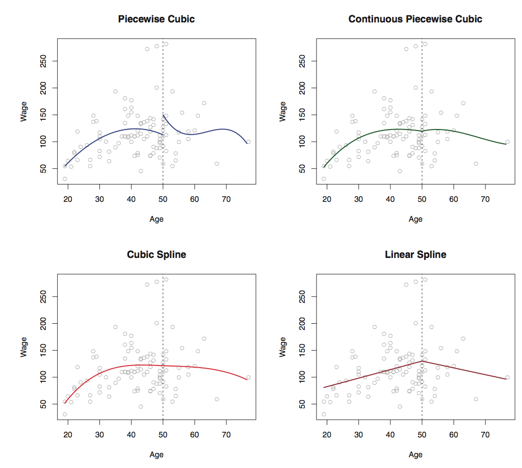
The only issue with this regression is Knot selection, but with improved libraries this issue is handled easily. Some common terms include:
- Linear splines - Piecewise linear polynomials continous at knots. In cubic spline, it is piecewise cubic polynomils
- Natural spline - According to John, it is fancier version of cubic splines. It adds constraints at the boundary which helps in extrapolating function linearly beyond the boundary knots.
With sayings of John, polynomials are more easy to think, but splines are much better behaved and more local.
References:
- Book - Statistics An introduction using R by Michael J. Crawley
- Book - An Intro to Statistical Learning by Gareth James et. al
- John, i.e., Trevor John Hastie, Professor at Stanford