Non-parametric Regression/Modelling

In parametric regression/modelling we set different parameters to model our data. Say if w know the underlying data distribution is normal then we can set different combination of mean and standard-deviations until the model will reflect underlying data perfectly. All right! But how will you model the data if you don't know the underlying data distribution. For example, in the below figure, underlying data distribution is uniform but on assuming that data is normal we got the estimate as shown, which is normal. This shows that we cannot rely on such parametric models if are not sure of underlying data distribution.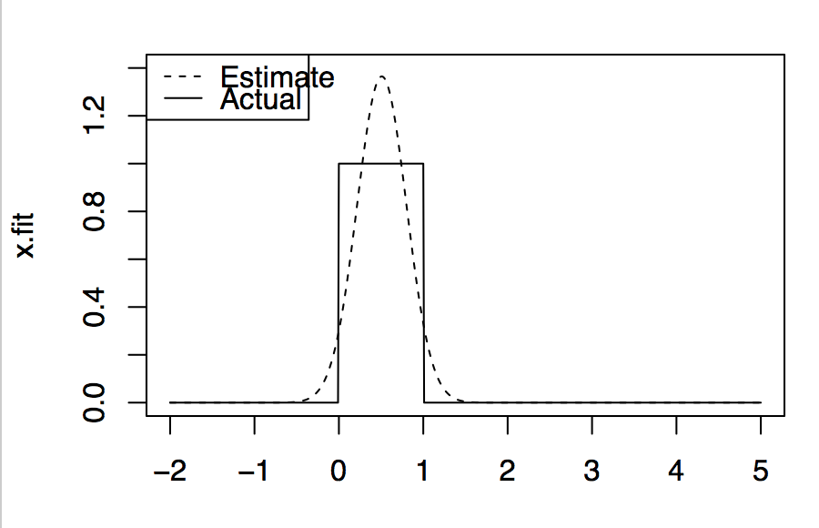

Non-Parametric Regression/Modelling or Kernel Density Estimation: In this, we use underlying data and some kernel function to model the data. The main idea is that at the point of interest we observe the neighboring points and  estimate value as a function of there positions/values. The neighboring points get weights according to kernel function used. The most common kernel function used is Gaussian kernel. Please find remaining  kernels used at this wiki link. An important tuning parameter in this technique is the width of the neighboring region considered for estimation, commonly known as bandwidth. This parameter controls the smoothness of estimation. Lower values results in more tightness but also include some noise, while as higher values result in more smoothness. But computing optimal value of bandwidth is not our concern as there exist number of approaches which calculate this value. The effect of bandwidth using  Gaussian kernel is shown in below figure.

This shows that automatic selection of bandwidth parameter is good enough to represent to underlying data distribution.

R code

[code language="CSS"]
set.seed(1988)
x = runif(700,min=0,max=1)
x.test = seq(-2,5,by=0.01)
x.fit = dnorm(x.test,mean(x),sd(x))
x.true = dunif(x.test,min=0,max=1)
bias = x.fit-x.true
#plot(bias~x.test)
plot(x.fit~x.test,t="l", ylim= c(0,1.4),lty=2)
lines(x.true~x.test,lty=1)
legend("topleft",legend = c("Estimate","Actual"), lty = c(2,1))
###########kernel density plots######
set.seed(1988)
ser = seq(-3,5, by=0.01)
x = c(rnorm(500,0,1),rnorm(500,3,1)) # mixture distributions
x.true = 0.5*dnorm(ser,0,1) + 0.5*dnorm(ser,3,1)
plot(x.true~ser,t="l")
par(mfrow=c(1,4))
# Guassian Kernel
plot(density(x,bw=0.1),ylim=c(0,0.3),lty=2, main="Gaussian Kernel, bw=0.1")
lines(x.true~ser,lty=1)
legend("topleft",legend = c("Actual","Estimated"),lty=c(1,2))

plot(density(x,bw=0.3),ylim=c(0,0.3),lty=2, main="Gaussian Kernel, bw=0.3")
lines(x.true~ser,lty=1)
legend("topleft",legend = c("Actual","Estimated"),lty=c(1,2))

plot(density(x,bw=0.8),ylim=c(0,0.3),lty=2, main="Gaussian Kernel, bw=0.8")
lines(x.true~ser,lty=1)
legend("topleft",legend = c("Actual","Estimated"),lty=c(1,2))

plot(density(x),ylim=c(0,0.3),lty=2, main="Gaussian Kernel, bw=automatic")
lines(x.true~ser,lty=1)
legend("topleft",legend = c("Actual","Estimated"),lty=c(1,2))

[/code]

References:

1. https://www.youtube.com/watch?v=QSNN0no4dSI
2. https://en.wikipedia.org/wiki/Kernel_(statistics)